1 2 3 4 5 6 7 / 7 7

Chapter 8. Calculation of shells of composite and with frames by the simplest method of "conjugation of sections of the integration interval".

Дата: 2025-05-25; Просмотры: 4

Оценка:

0.00 из 5.00 — оценок

Скачиваний: 0

8.1. The variant of recording of the method for solving stiff boundary value problems without orthonormalization - the method of "conjugation of sections, expressed by matrix exponents "- with positive directions of matrix formulas of integration of differential equations.

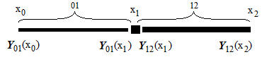
We divide the interval of integration of the boundary value problem, for example, into 3 sections. We will have points (nodes), including edges:

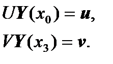
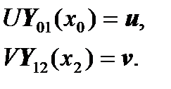
We have boundary conditions in the form:

We can write the matrix equations of conjugation of sections:

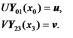
We can rewrite it in a form more convenient for us further:

where is the identity matrix.

As a result, we obtain a system of linear algebraic equations:

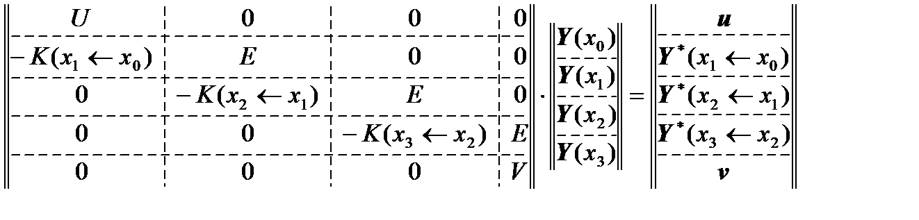This system is solved by Gauss’ method with the separation of the main element.

It turns out that it is not necessary to apply orthonormalization, since sections of the integration interval are chosen so long that the computation on them is stable.

At points near the nodes, the solution is found by solving the corresponding Cauchy’s problems with the origin at the i-th node:

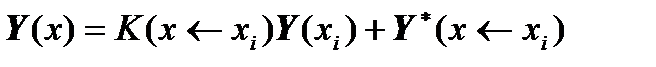8.2. Composite shells of rotation.

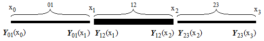
Let us consider the conjugation of segments of the composite shell of rotation.

Suppose we have 3 sections, where each section can be expressed by its differential equations and the physical parameters can be expressed differently - different formulas on different sections:

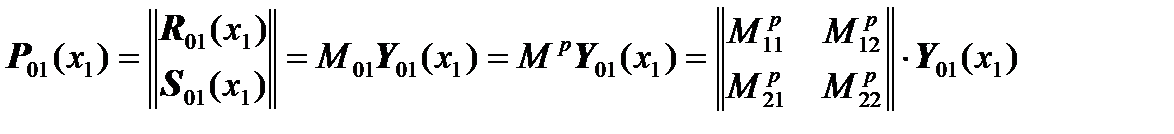
In the general case (for the example of section 12), the physical parameters of the section (vector ) are expressed in terms of the required parameters of the system of ordinary differential equations of this section (through the vector ) as follows:

where the matrix is a square non-degenerate matrix.

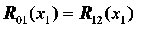
With the transition of the conjugation point, we can write in a general form (but using the conjugation point ):

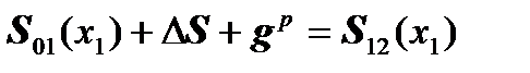
where is the discrete increment of physical parameters (forces, moments) during the transition from the "01" section to the "12" section, and the square nondegenerate matrix is diagonal and consists of units and minus ones on the main diagonal to establish the correct correspondence between the positive directions of forces, angular momenta, displacements and angles when going from "01" to "12", which may be different (in different differential equations of different conjugate regions) in the equations to the left of the conjugation point and in the equations to the right of the conjugation point.

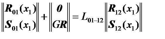
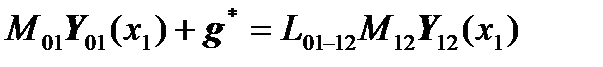
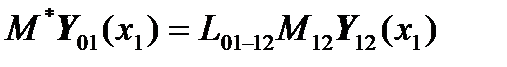
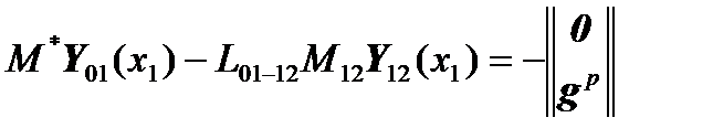
The last two equations combine to form the equation:

At the conjugation point , we similarly obtain the equation:

If the shell consisted of identical parts, then we could write in a combined matrix form a system of linear algebraic equations in the following form:

But in our case the shell consists of 3 sections, where the middle section can be considered, for example, a frame expressed in terms of its differential equations.

Then instead of vectors , , , we should consider vectors:

Then the matrix equations

will take the form:

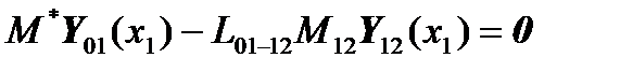
After rearranging the summands, we get:

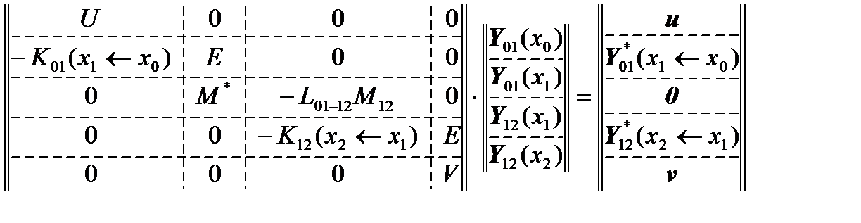
As a result, we can write down the final system of linear algebraic equations:

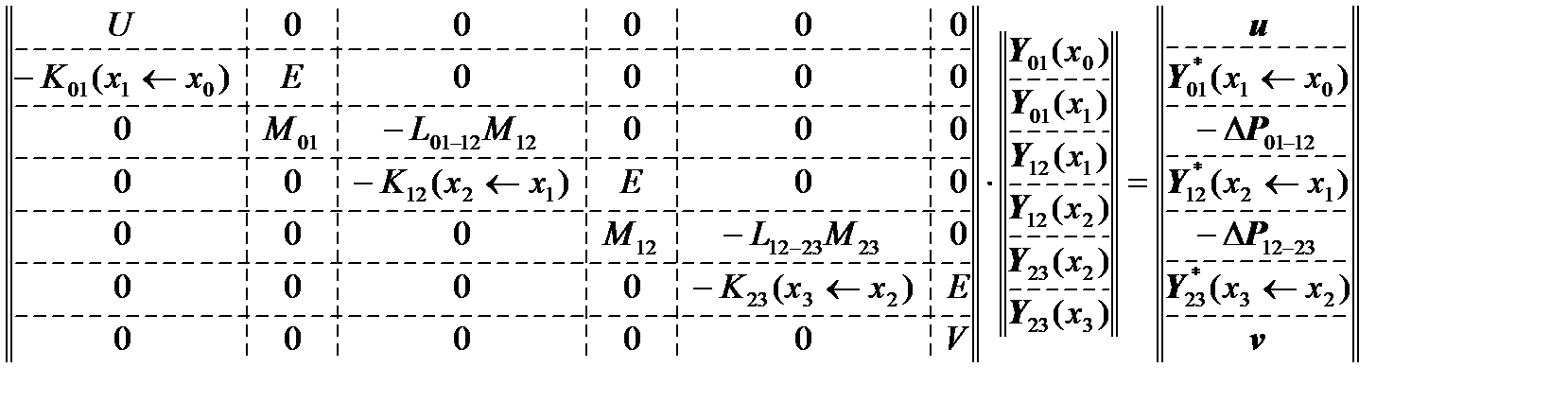
This system is solved by the Gauss method with the separation of the main element.

At points located between nodes, the solution is to be solved by solving Cauchy’s problems with the initial conditions in the i-th node:

It is not necessary to apply orthonormalization for boundary value problems for stiff ordinary differential equations.

8.3. Frame, expressed not by differential, but algebraic equations.

Let us consider the case when the frame (at a point ) is expressed not in terms of differential equations, but in terms of algebraic equations.

Above we wrote down that:

We can represent the vector of force factors and displacements in the form:

where is the displacement vector, is the vector of forces and moments.

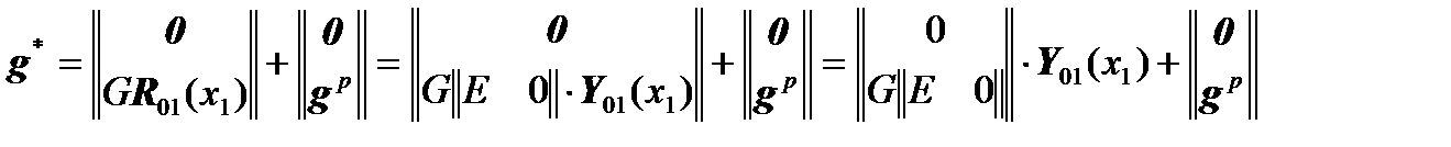
Algebraic equation for the frame:

where G is the matrix of the rigidity of the frame, R is the vector of the frame movements, is the vector of force factors that act on the frame.

At the point of the frame we have:

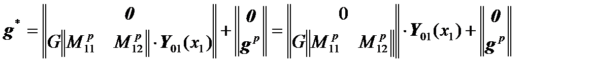
that is, there is no discontinuity in the movements , but there is a resultant vector of force factors , which consists of forces and moments on the left plus forces and moments to the right of the point of the frame.

, где ,

which is true if we do not forget that in this case we have:

that is, the vector of displacements and force factors is first compiled from displacements (above) , and then from force factors (below) .

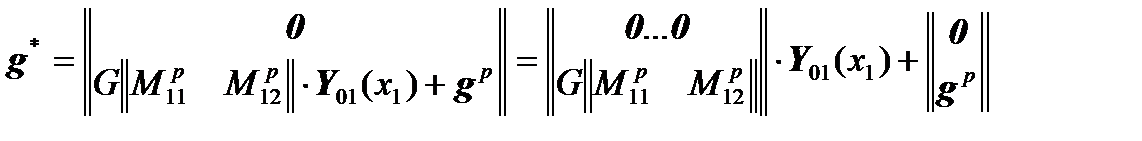
Here it is necessary to remember that the displacement vector is expressed in terms of the required state vector :

where for convenience was introduced re-designation .

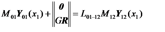
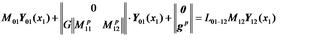
Then we can write:

We write the matrix equations for this case:

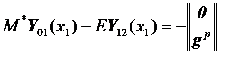
Let us write the vector in the equation:

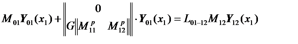To ensure the non-cumbersomeness, we introduce the notation:

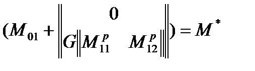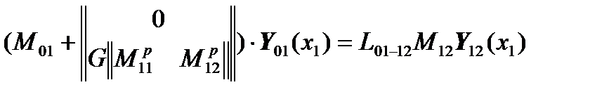
Then equation

will take the form:

For convenience, we rearrange the terms in the matrix equations so that the resulting system of linear algebraic equations is written clearly:

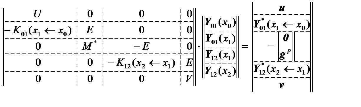
Thus, we obtain the resulting system of linear algebraic equations:

If an external force-moment action is applied to the frame, then

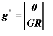
should be rewritten in the form 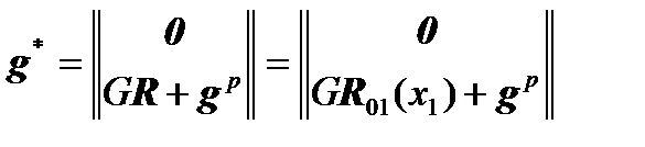, then:

Then the matrix equation

will take the form:

The resulting system of linear algebraic equations takes the form:

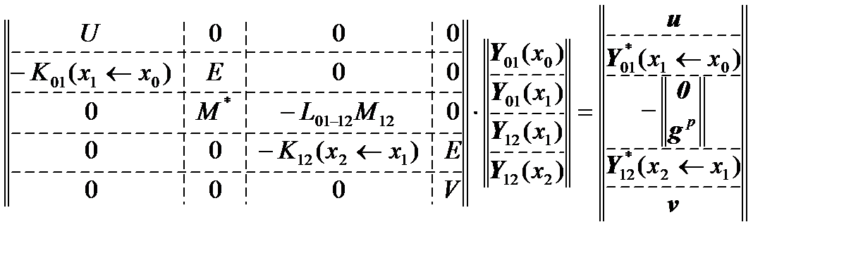8.4. The case where the equations (of shells and frames) are expressed not with abstract vectors, but with vectors, consisting of specific physical parameters.

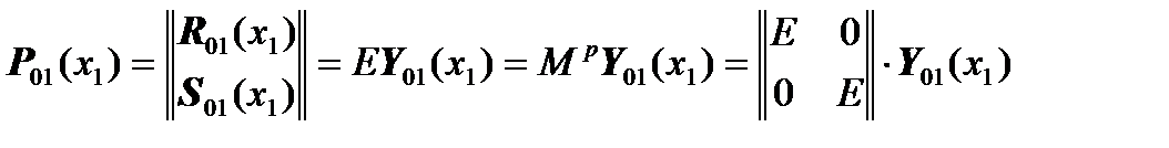
Let us consider the case when the parts of the shell structure and the frame are expressed with state vectors (such as ), which (in a particular case) coincide with vectors of physical parameters (such as - displacements, angles, forces, moment). Then the matrices of type are unit: . And let the positive directions of the physical parameters be the same for all parts of the shell and the frame ( ).

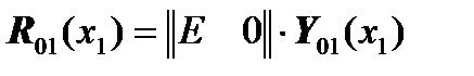
Then we have the equations:

as:

where E is the identity matrix.

Equations

will take the form:

Equations

will take the form:

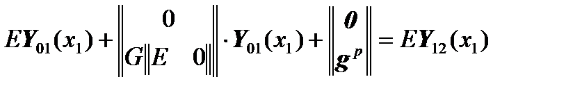, где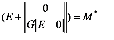

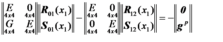
The resulting system of linear algebraic equations

will take the form:

where .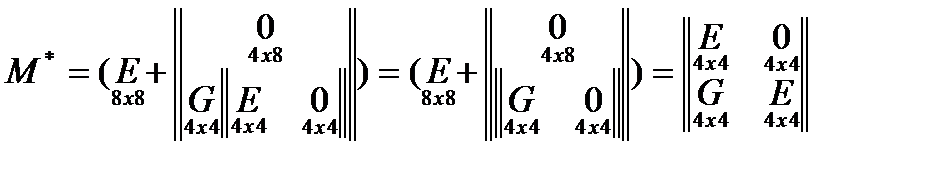

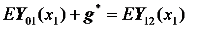
This means that equation

will take the form:

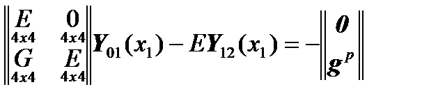
, (there is no jump in the displacements and the angle) and

- base balance,

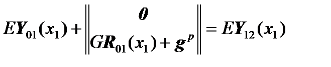
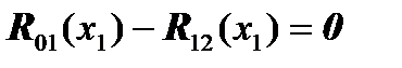
i.e:

(displacement and angle: no rupture)

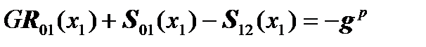
, где 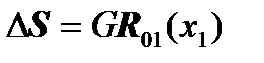(strength and momentum: balance).

Appendix. Computational experiments (a C++ program).

Computational experiments have been carried out in comparison with the method of the boundary conditions transfer of Alexei Vinogradov. Line-by-line orthonormalization is used in this method.

Without use of orthonormalization it is possible by means of the boundary conditions transfer method to solve a problem of cylindrical shell loading that is fixed in cantilever fashion at the right boundary and loaded at the left boundary by the force distributed uniformly by the circular arch with the ratio of the length to the radius L/R=2 and with ratio of the radius to the thickness R/h=100. In case of ratio R/h=200 the problem by means of the method of the boundary conditions transfer without orthonormalozation cannot be solved by this time because there are mistakes resulted in due to counting instability. However, in case of use of orthonormalization in the method of the boundary conditions transfer the problems related to the parameters R/h=300, R/h=500, R/h=1000 can be solved.

A new method proposed in this paper allows solving of all above mentioned test problems without use of orthonormalization operation that results in significant simplification of its programming.

In case of the test computations of the problems characterized by the above mentioned parameters by means of this new proposed method the integration interval is divided into 10 segments while between the nodes as aforesaid the solution was found as a solution of Cauchy’s problem. 50 harmonics of Fourier’s series were used for solving the problem since the result in case of usage of 50 harmonics didn’t differ from the case when 100 harmonics were used.

Test problem computing speed by means of the proposed method is not less compared to the boundary conditions transfer method because both methods when used for test problems while using 50 harmonics of the Fourier series produced a final solution instantaneously after launching a program (notebook ASUS M51V CPU Duo T5800). At the same time programming of this newly proposed method is significantly simpler because there is no need in orthonormalization procedure programming.

C++ program

// sopryazhenie.cpp: main file of the project.

//Solution of the boundary value problem – a cylindrical shell problem.

//Integration interval is divided into 10 matching segments: left boundary – point 0 and right boundary – point 10.

//WITHOUT ORTHONORMALIZATION

#include "stdafx.h"

#include <iostream>

#include <conio.h>

using namespace std;

//Multiplication of A matrix by b vector and obtain rezult.

void mat_on_vect(double A[8][8], double b[8], double rezult[8]){

for(int i=0;i<8;i++){

rezult[i]=0.0;

for(int k=0;k<8;k++){

rezult[i]+=A[i][k]*b[k];

}

//Computation of the matrix exponent EXP=exp(A*delta_x)

void exponent(double A[8][8], double delta_x, double EXP[8][8]) {

//n – number of the terms of the series in the exponent, m – a counter of the number of the terms of the series (m<=n)

int n=100, m;

double E[8][8]={0}, TMP1[8][8], TMP2[8][8];

int i,j,k;

//E – unit matrix – the first term of the series of the exponent

E[0][0]=1.0; E[1][1]=1.0; E[2][2]=1.0; E[3][3]=1.0;

E[4][4]=1.0; E[5][5]=1.0; E[6][6]=1.0; E[7][7]=1.0;

//initial filling-in of the auxiliary array TMP1 – the previous term of the series for follow-up multiplication

//and initial filling-in of the exponent by the first term of the series

for(i=0;i<8;i++) {

for(j=0;j<8;j++) {

TMP1[i][j]=E[i][j];

EXP[i][j]=E[i][j];

}

//series of EXP exponent computation starting from the 2^nd term of the series (m=2;m<=n)

for(m=2;m<=n;m++) {

for(i=0;i<8;i++) {

for(j=0;j<8;j++) {

TMP2[i][j]=0;

for(k=0;k<8;k++) {

//TMP2[i][j]+=TMP1[i][k]*A[k][j]*delta_x/(m-1);

TMP2[i][j]+=TMP1[i][k]*A[k][j];

}

TMP2[i][j]*=delta_x;//taken out beyond the cycle of multiplication of the row by the column

TMP2[i][j]/=(m-1);// taken out beyond the cycle of multiplication of the row by the column

EXP[i][j]+=TMP2[i][j];

}

//filling-in of the auxiliary array TMP1 for computing the next term of the series TMP2 in the next step of the cycle by m

if (m<n) {

for(i=0;i<8;i++) {

for(j=0;j<8;j++) {

TMP1[i][j]=TMP2[i][j];

}

//computation of the matrix MAT_ROW in the form of the matrix series for follow-up use

//when computing a vector - partial vector – a vector of the partial solution of the heterogeneous system of the ordinary differential equations at the step delta x

void mat_row_for_partial_vector(double A[8][8], double delta_x, double MAT_ROW[8][8]) {

//n – number of the terms of the series in MAT_ROW, m – a counter of the number of the terms of the series (m<=n)

int n=100, m;

double E[8][8]={0}, TMP1[8][8], TMP2[8][8];

int i,j,k;

//E – unit matrix – the first term of the series MAT_ROW

E[0][0]=1.0; E[1][1]=1.0; E[2][2]=1.0; E[3][3]=1.0;

E[4][4]=1.0; E[5][5]=1.0; E[6][6]=1.0; E[7][7]=1.0;

//initial filling-in of the auxiliary array TMP1 – the previous term of the series for following multiplication

//and initial filling-in of MAT_ROW by the first term of the series

for(i=0;i<8;i++) {

for(j=0;j<8;j++) {

TMP1[i][j]=E[i][j];

MAT_ROW[i][j]=E[i][j];

}

//a series of computation of MAT_ROW starting from the second term of the series (m=2;m<=n)

for(m=2;m<=n;m++) {

for(i=0;i<8;i++) {

for(j=0;j<8;j++) {

TMP2[i][j]=0;

for(k=0;k<8;k++) {

TMP2[i][j]+=TMP1[i][k]*A[k][j];

}

TMP2[i][j]*=delta_x;

TMP2[i][j]/=m;

MAT_ROW[i][j]+=TMP2[i][j];

}

//filling-in of the auxiliary array TMP1 for computing the next term of the series – TMP2 in the next step of the cycle by m

if (m<n) {

for(i=0;i<8;i++) {

for(j=0;j<8;j++) {

TMP1[i][j]=TMP2[i][j];

}

//specifying the external influence vector in the system of ordinary differential equations – POWER vector: Y'(x)=A*Y(x)+POWER(x):

void power_vector_for_partial_vector(double x, double POWER[8]){

POWER[0]=0.0;

POWER[1]=0.0;

POWER[2]=0.0;

POWER[3]=0.0;

POWER[4]=0.0;

POWER[5]=0.0;

POWER[6]=0.0;

POWER[7]=0.0;

}

//computation of the vector – ZERO (particular case) vector of the partial solution

//heterogeneous system of differential equations in the segment of interest:

void partial_vector(double vector[8]){

for(int i=0;i<8;i++){

vector[i]=0.0;

}

//computation of the vector – the vector of the partial solution of the heterogeneous system of differential equations in the segment of interest delta x:

void partial_vector_real(double expo_[8][8], double mat_row[8][8], double

x_, double delta_x, double vector[8]){

double POWER_[8]={0};//External influence vector on the shell

double REZ[8]={0};

double REZ_2[8]={0};

power_vector_for_partial_vector(x_, POWER_);//Computing POWER_ at coordinate x_

mat_on_vect(mat_row, POWER_, REZ);//Multiplication of the matrix mat_row by POWER vector and obtain REZ vector

mat_on_vect(expo_, REZ, REZ_2);// Multiplication of matrix expo_ by vector REZ and obtain vector REZ_2

for(int i=0;i<8;i++){

vector[i]=REZ_2[i]*delta_x;

}

//Solution of SLAE of 88 dimensionality by the Gauss method with discrimination of the basic element

int GAUSS(double AA[8*11][8*11], double bb[8*11], double x[8*11]){

double A[8*11][8*11];

double b[8*11];

for(int i=0;i<(8*11);i++){

b[i]=bb[i];//we will operate with the vector of the и right parts to provide that initial vector bb would not change when exiting the subprogram

for(int j=0;j<(8*11);j++){

A[i][j]=AA[i][j];//we will operate with A matrix to provide that initial AA matrix would not change when exiting the subprogram

}

int e;//number of the row where main (maximal) coefficient in the column jj is found

double s, t, main;//Ancillary quantity

for(int jj=0;jj<((8*11)-1);jj++){//Cycle by columns jj of transformation of A matrix into upper-triangle one

e=-1; s=0.0; main=A[jj][jj];

for(int i=jj;i<(8*11);i++){//there is a number of у row where main (maximal) element is placed in the column jj and row interchanging is made

if ((A[i][jj]*A[i][jj])>s) {//Instead of multiplication (potential minus sign is deleted) it could be possible to use a function by abs() module

e=i; s=A[i][jj]*A[i][jj];

}

if (e<0) {

cout<<"Mistake "<<jj<<"\n"; return 0;

}

if (e>jj) {//If the main element isn’t placed in the row with jj number but is placed in the row with у number

main=A[e][jj];

for(int j=0;j<(8*11);j++){//interchanging of two rows with e and jj numbers

t=A[jj][j]; A[jj][j]=A[e][j]; A[e][j]=t;

}

t=b[jj]; b[jj]=b[e]; b[e]=t;

}

for(int i=(jj+1);i<(8*11);i++){//reduction to the upper-triangle matrix

for(int j=(jj+1);j<(8*11);j++){

A[i][j]=A[i][j]-(1/main)*A[jj][j]*A[i][jj];//re-calculation of the coefficients of the row i>(jj+1)

}

b[i]=b[i]-(1/main)*b[jj]*A[i][jj];

A[i][jj]=0.0;//nullified elements of the row under diagonal element of A matrix

}

}//Cycle by jj columns of transformation of A matrix into upper-triangle one

x[(8*11)-1]=b[(8*11)-1]/A[(8*11)-1][(8*11)-1];//initial determination of the last element of the desired solution x (87^th)

for(int i=((8*11)-2);i>=0;i--){//Computation of the elements of the solution x[i] from 86^th to 0^th

t=0;

for(int j=1;j<((8*11)-i);j++){

t=t+A[i][i+j]*x[i+j];

}

x[i]=(1/A[i][i])*(b[i]-t);

}

return 0;

}

int main()

{

int nn;//Number of the harmonic starting from the 1^st (without zero one)

int nn_last=50;//Number of the last harmonic

double Moment[100+1]={0};//An array of the physical parameter (momentum) that is computed in each point between the boundaries

double step=0.05; //step=(L/R)/100 – step size of shell computation – a step of integration interval (it should be over zero, i.e. be positive)

double h_div_R;//Value of h/R

h_div_R=1.0/100;

double c2;

c2=h_div_R*h_div_R/12;//Value of h*h/R/R/12

double nju;

nju=0.3;

double gamma;

gamma=3.14159265359/4;//The force distribution angle by the left boundary

//printing to files:

FILE *fp;

// Open for write

if( (fp = fopen( "C:/test.txt", "w" )) == NULL ) // C4996

printf( "The file 'C:/test.txt' was not opened\n" );

else

printf( "The file 'C:/test.txt' was opened\n" );

for(nn=1;nn<=nn_last;nn++){ //A CYCLE BY HARMONICS STARTING FROM THE 1^st HARMONIC (EXCEPT ZERO ONE)

double x=0.0;//A coordinate from the left boundary – it is needed in case of heterogeneous system of the ODE for computing the particular vector FF

double expo_from_minus_step[8][8]={0};//The matrix for placement of the exponent in it at the step of (0-x1) type

double expo_from_plus_step[8][8]={0};// The matrix for placement of the exponent in it in the step of (x1-0) type

double mat_row_for_minus_expo[8][8]={0};//the auxiliary matrix for particular vector computing when moving at step of (0-x1) type

double mat_row_for_plus_expo[8][8]={0};// the auxiliary matrix for particular vector computing when moving at step of (x1-0) type

double U[4][8]={0};//The matrix of the boundary conditions of the left boundary of the dimensionality 4x8

double u_[4]={0};//Dimensionality 4 vector of the external influence for the boundary conditions of the left boundary

double V[4][8]={0};//The boundary conditions matrix of the right boundary of the dimensionality 4x8

double v_[4]={0};// The dimensionality 4 vector of the external influence for the boundary conditions for the right boundary

double Y[100+1][8]={0};//The array of the vector-solutions of the corresponding linear algebraic equations system (in each point of the interval between the boundaries): MATRIXS*Y=VECTORS

double A[8][8]={0};//Matrix of the coefficients of the system of ODE

double FF[8]={0};//Vector of the particular solution of the heterogeneous ODE at the integration interval sector

double Y_many[8*11]={0};// a composite vector consisting of the vectors Y(xi) in 11 points from point 0 (left boundary Y(0) to the point 10 (right boundary Y(x10))

double MATRIX_many[8*11][8*11]={0};//The matrix of the system of the linear algebraic equations

double B_many[8*11]={0};// a vector of the right parts of the SLAE: MATRIX_many*Y_many=B_many

double Y_vspom[8]={0};//an auxiliary vector

double Y_rezult[8]={0};//an auxiliary vector

double nn2,nn3,nn4,nn5,nn6,nn7,nn8;//Number of the nn harmonic raised to corresponding powers

nn2=nn*nn; nn3=nn2*nn; nn4=nn2*nn2; nn5=nn4*nn; nn6=nn4*nn2; nn7=nn6*nn; nn8=nn4*nn4;

//Filling-in of non-zero elements of the A matrix of the coefficients of ODE system

A[0][1]=1.0;

A[1][0]=(1-nju)/2*nn2; A[1][3]=-(1+nju)/2*nn; A[1][5]=-nju;

A[2][3]=1.0;

A[3][1]=(1+nju)/(1-nju)*nn; A[3][2]=2*nn2/(1-nju); A[3][4]=2*nn/(1-nju);

A[4][5]=1.0;

A[5][6]=1.0;

A[6][7]=1.0;

A[7][1]=-nju/c2; A[7][2]=-nn/c2; A[7][4]=-(nn4+1/c2); A[7][6]=2*nn2;

//Here firstly it is necessary to make filling-in by non-zero values of the matrix and boundary conditions vector U*Y[0]=u_ (on the left) and V*Y[100]=v_ (on the right):

U[0][1]=1.0; U[0][2]=nn*nju; U[0][4]=nju; u_[0]=0.0;//Force T1 at the left boundary is equal to zero

U[1][0]=-(1-nju)/2*nn; U[1][3]=(1-nju)/2; U[1][5]=(1-nju)*nn*c2; u_[1]=0.0;//Force S* at the left boundary is equal to zero

U[2][4]=-nju*nn2; U[2][6]=1.0; u_[2]=0;//Momentum M1 at the left boundary is equal to zero

U[3][5]=(2-nju)*nn2; U[3][7]=-1.0;

u_[3]=-sin(nn*gamma)/(nn*gamma);//Force Q1* at the left boundary is distributed at the angle -gamma +gamma

V[0][0]=1.0; v_[0]=0.0;// The right boundary displacement u is equal to zero

V[1][2]=1.0; v_[1]=0.0;//The right boundary displacement v is equal to zero

V[2][4]=1.0; v_[2]=0.0;//The right boundary displacement w is equal to zero

V[3][5]=1.0; v_[3]=0.0;//The right boundary rotation angle is equal to zero

//Here initial filling-in of U*Y[0]=u_ и V*Y[100]=v_ terminates

exponent(A,(-step*10),expo_from_minus_step);//A negative step (step value is less than zero due to direction of matrix exponent computation)

//x=0.0;//the initial value of coordinate – for partial vector computation

//mat_row_for_partial_vector(A, step, mat_row_for_minus_expo);

//Filling-in of the SLAE coefficients matrix MATRIX_many

for(int i=0;i<4;i++){

for(int j=0;j<8;j++){

MATRIX_many[i][j]=U[i][j];

MATRIX_many[8*11-4+i][8*11-8+j]=V[i][j];

}

B_many[i]=u_[i];

B_many[8*11-4+i]=v_[i];

}

for(int kk=0;kk<(11-1);kk++){//(11-1) unit matrix and EXPO matrix should be written into MATRIX_many

for(int i=0;i<8;i++){

MATRIX_many[i+4+kk*8][i+kk*8]=1.0;//filling-in by unit matrixes

for(int j=0;j<8;j++){

MATRIX_many[i+4+kk*8][j+8+kk*8]=-expo_from_minus_step[i][j];//filling-in by matrix exponents

}

//Solution of the system of linear algebraic equations

GAUSS(MATRIX_many,B_many,Y_many);

//Computation of the state vectors in 101 points – left point 0 and right point 100

exponent(A,step,expo_from_plus_step);

for(int i=0;i<11;i++){//passing points filling-in in all 10 intervals (we will obtain points from 0 to 100) between 11 nodes

for(int j=0;j<8;j++){

Y[0+i*10][j]=Y_many[j+i*8];//in 11 nodes the vectors are taken from SLAE solutions – from Y many

}

for(int i=0;i<10;i++){//passing points filling-in in 10 intervals

for(int j=0;j<8;j++){

Y_vspom[j]=Y[0+i*10][j];//the initial vector for i^th segment, zero point, starting point of the i^th segment

}