
Chapter 5. The method of "half of the constants" for solving boundary value problems with non-stiff ordinary differential equations.


In this method we use the idea proposed by S.K.Godunov to seek a solution in the form of only one-half of the possible unknown constants, but a formula for the possibility of starting such a calculation and further application of matrix exponents (Cauchy’s matrices) are proposed by A.Yu.Vinogradov.
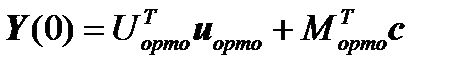
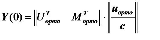
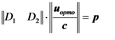
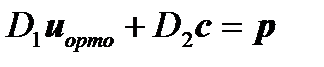
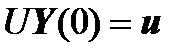
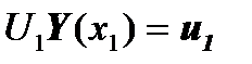
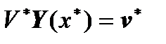
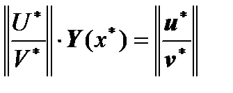
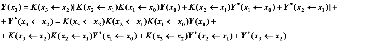
The formula for starting calculations from the left edge with only one half of the possible constants:
 ,
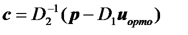
,
 .
.
Thus, a formula is written in the matrix form for the beginning of the calculation from the left edge, when the boundary conditions are satisfied on the left edge.
Then write  and
and 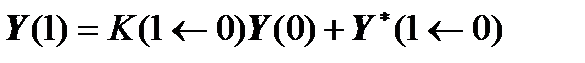 collectively:
 ,
,
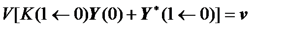
and substitute in this formula the expression for Y(0):
or
 .
.
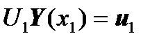
Thus, we have obtained an expression of the form:
 ,
,
where the matrix  has a dimension of 4x8 and can be naturally represented in the form of two square blocks of 4x4 dimension:
 .
.
Then we can write:
 .
.
Hence we obtain that:
 .
.
Thus, the required constants are found.
Chapter 6. The method of "transferring of boundary conditions" (step-by-step version of the method) for solving boundary value problems with stiff ordinary differential equations.
6.1. The method of "transfer of boundary value conditions" to any point of the interval of integration.
The complete solution of the system of differential equations has the form
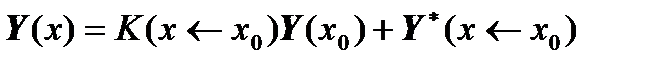 .
.
Or you can write:
 .
.
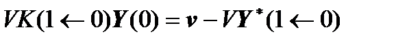
We substitute this expression for  into the boundary conditions of the left edge and obtain:
 ,
,
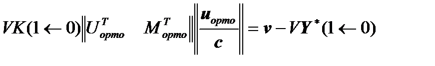
 ,
,
 .
.
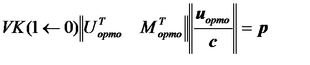
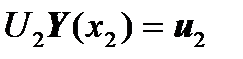
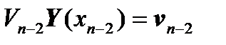
Or we get the boundary conditions transferred to the point  :
:
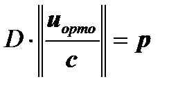
 ,
,
where 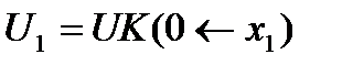 and
and 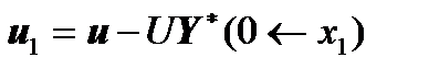 .
.
Further, we write similarly

And substitute this expression for  into the transferred boundary conditions of the point
  :
:
 ,
,
 ,
,
 .
.
Or we get the boundary conditions transferred to the point  :
:
 ,
,
where 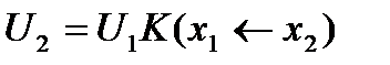 and
and 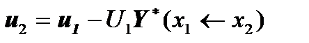 .
.
And so we transfer the matrix boundary condition from the left edge to the point  and in the same way transfer the matrix boundary condition from the right edge.
Let us show the steps of transferring the boundary conditions of the right edge.
We can write:

We substitute this expression for  in the boundary conditions of the right edge and obtain:
 ,
,
 ,
,

Or we get the boundary conditions of the right edge, transferred to the point  :
:
 ,
,
where  and
and  .
.
Further, we write similarly

And substitute this expression for  in the transferred boundary conditions of the point
  :
:
,
 ,
,
 .
.
Or we get the boundary conditions transferred to the point  :
:
 ,
,
where 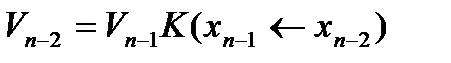 and
and 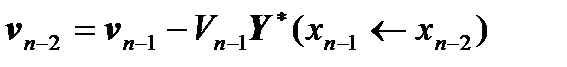 .
.
And so at the inner point of the integration interval we transfer the matrix boundary condition, as shown, and from the left edge and in the same way transfer the matrix boundary condition from the right edge and obtain:
 ,
,
 .
.
From these two matrix equations with rectangular horizontal coefficient matrices, we obviously obtain one system of linear algebraic equations with a square matrix of coefficients:
 .
.
6.2. The case of "stiff" differential equations.
In the case of "stiff" differential equations, it is proposed to apply a line orthonormalization of the matrix boundary conditions in the process of their transfer to the point under consideration. For this, the orthonormalization formulas for systems of linear algebraic equations can be taken in [Berezin, Zhidkov].
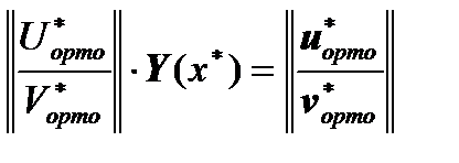
That is, having received
we apply a line orthonormation to this group of linear algebraic equations and obtain an equivalent matrix boundary condition:
 .
.
And in this line orthonormal equation is substituted
 .
.
And we get
 ,
,
 .
.
Or we get the boundary conditions transferred to the point :
,
where  and
and 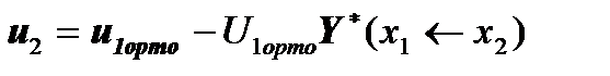 .
.
Now we apply linear orthonorming to this group of linear algebraic equations and obtain an equivalent matrix boundary condition:

And so on.
And similarly we do with intermediate matrix boundary conditions carried from the right edge to the point under consideration.
As a result, we obtain a system of linear algebraic equations with a square matrix of coefficients, consisting of two independently stepwise orthonormal matrix boundary conditions, which is solved by Gauss’ method with the separation of the main element for obtaining the solution  at the point
  under consideration:
 .
.
6.3. Formulas for computing the vector of a particular solution of inhomogeneous system of differential equations.
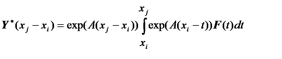
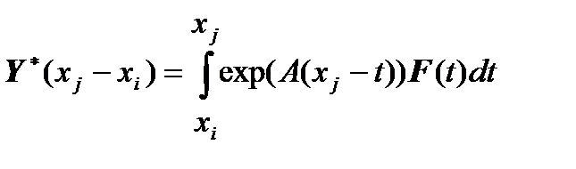
Instead of the formula for computing the vector of a particular solution of an inhomogeneous system of differential equations in the form [Gantmaher]:
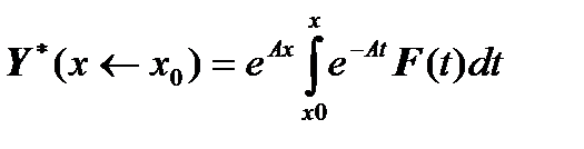
it is proposed to use the following formula for each individual section of the integration interval:
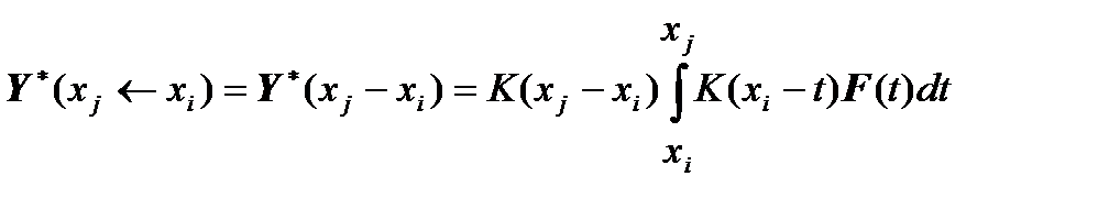 .
.
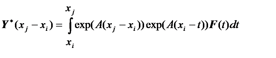
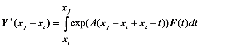
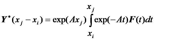
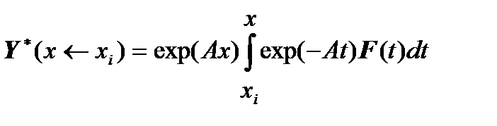
The correctness of the above formula is confirmed by the following:
 ,
,
 ,
,
 ,
,
 ,
,
 ,
,
 ,
,
which was to be confirmed.
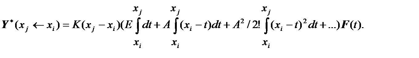
The calculation of the vector of a particular solution of a system of differential equations is performed using the representation of Cauchy’s matrix under the integral sign in the form of a series and integrating this series elementwise:
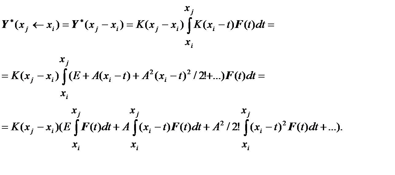
This formula is valid for the case of a system of differential equations with constant coefficient matrix  =const.
Let us consider the variant, when the steps of the integration interval are chosen sufficiently small, which allows us to consider the vector  in the region
  approximately as a constant
  , which allows us to remove this vector from the signs of the integrals:
It is known that when T=(at+b) we have 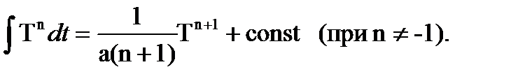
In our case, we have 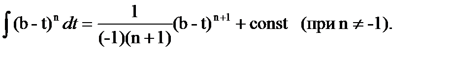
Then we obtain 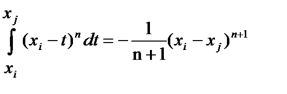 .
.
Then we obtain a series for computing the vector of a particular solution of an inhomogeneous system of differential equations on a small section :

For the case of differential equations with variable coefficients, an averaged matrix  of the coefficients of the system of differential equations can be used for each section.
If the considered section of the integration interval is not small, then the following iterative (recurrent) formulas are proposed.
We give the formulas for computing the vector of a particular solution, for example,  on the considered section
  through the vectors of the particular solution
  ,
,  ,
,  , corresponding to the subsections
  ,
,  ,
,  .
.
We have .
We also have a formula for a separate subsection:
.
We can write:
 ,
,
 .
.
We substitute  in
in  and get:

 .
.
Let us compare the expression obtained with the formula:

and we get, obviously, that:

and for the particular vector we obtain the formula:
 .
.
That is, the subsector vectors 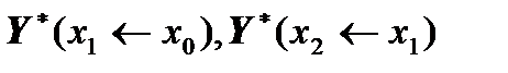 are not simply add with each other, but with the participation of Cauchy’s matrix of the subsection.
Similarly, we write down  and substitute the formula for
  and get:
Comparing the expression obtained with the formula:

obviously, we get that:

and together with this we get the formula for a particular vector:
That is, in this way a particular vector is calculated - the vector of the particular solution of the inhomogeneous system of differential equations, that is, for example, a particular vector on the considered section is calculated through the computed partial vectors , , corresponding to the sub-sections , , .
6.4. Applicable formulas for orthonormalization.
Taken from [Berezin, Zhidkov]. Let there be given a system of linear algebraic equations of order n:

 =
=  .
.
Here, above the vectors, we draw dashes instead of their designation in boldface.
We will consider the rows of the matrix  of the system as vectors:
 =(
=(  ,
,  ,…,
,…,  ).
).
We orthonormalize this system of vectors.
The first equation of the system = we divide by  .
.
In doing so, we get:

 +
+ 
 +…+
+…+ 
 =
=  ,
,  =(
=(  ,
,  ,…,
,…,  ),
),
where  =
=  ,
,  =
=  ,
,  =1.
=1.
The second equation of the system is replaced by:
 +
+  +…+
+…+  =
=  ,
,  =(
=(  ,
,  ,…,
,…,  ),
),
where  =
=  ,
,  =
=  ,
,
 =
=  -(
-(  ,
,  )
)  ,
,  =
=  -( ,
-( ,  )
)  .
.
Similarly we proceed further. The equation with the number i takes the form:
 +
+  +…+
+…+  =
=  ,
,  =(
=(  ,
,  ,…,
,…,  ),
),
where  =
=  ,
,  =
=  ,
,
 =
=  -(
-(  , ) -(
  ,
,  )
)  -…-( ,
  )
)  ,
,
 =
=  -( , ) -( , )
  -…-( , )
  .
.
Here ( ,  ) is the scalar multiplication of vectors.
The process will be realized if the system of linear algebraic equations is linearly independent.
As a result, we come to a new system  , where the matrix
  will be with orthonormal rows, that is, it has the property
  , where
  is the identity matrix.
Chapter 7. The simplest method for solving boundary value problems with stiff ordinary differential equations without orthonormalization - the method of "conjugation of sections of the integration interval", which are expressed by matrix exponents.
The idea of overcoming the difficulties of computation by dividing the interval of integration into conjugate areas belongs to Dr.Sc. Professor Yu.I.Vinogradov (his doctoral thesis was defended including on this idea), and the simplest realization of this idea through the formulas of the theory of matrices belongs to the Ph.D. A.Yu.Vinogradov.
We divide the interval of integration of the boundary value problem, for example, into 3 sections. We will have points (nodes), including edges:
 .
.
We have boundary conditions in the form:
We can write the matrix equations of conjugation of sections:
 ,
,
 ,
,
 .
.
We can rewrite it in a form more convenient for us further:
 ,
,
 ,
,
 .
.
where  is the identity matrix.
Then in a combined matrix form we obtain a system of linear algebraic equations in the following form:
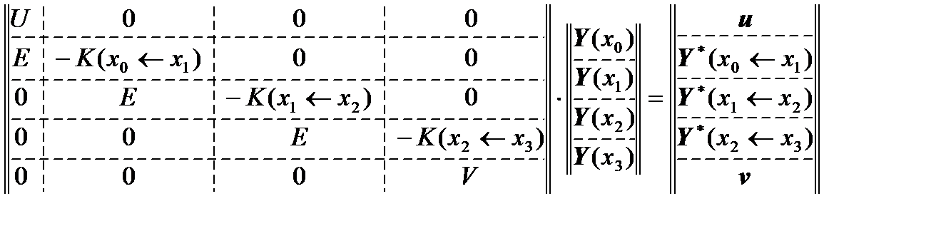 .
.
This system is solved by Gauss’ method with the separation of the main element.
At points located between nodes, the solution is to be solved by solving Cauchy’s problems with the initial conditions in the i-th node:
 .
.
It is not necessary to apply orthonormalization for boundary value problems for stiff ordinary differential equations, since on each section of the integration interval the calculation of each matrix exponent is fulfilled independently and from the initial orthonormal identity matrix, which makes it unnecessary to use orthonormalization, unlike S.K.Godunov’s method, which greatly simplifies programming in comparison with S.K.Godunov's method.
It is possible to calculate Cauchy’s matrices not in the form of matrix exponents, but with Runge-Kutta’s methods from the starting identity matrix, and the vector of the particular solution of the inhomogeneous system of differential equations can be calculated on each site by Runge-Kutta’s methods from the starting zero vector. In the case of Runge-Kutta’s methods, error estimates are well known, which means that calculations can be performed with a known accuracy.