
Chapter 3. The method of "transferring of boundary value conditions" (the direct version of the method) for solving boundary value problems with non-stiff ordinary differential equations.


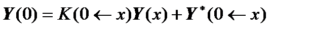
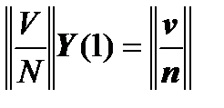
It is proposed to integrate by the formulas of the theory of matrices [Gantmakher] immediately from some inner point of the interval of integration to the edges:
 ,
,
 .
.
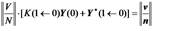
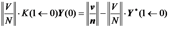
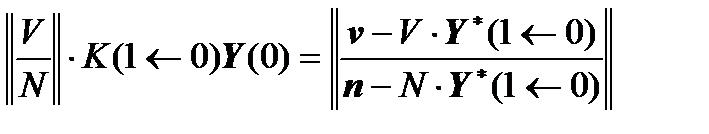
We substitute the formula for  in the boundary conditions of the left edge and obtain:
 ,
,
 ,
,
 .
.
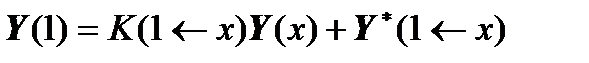
Similarly, for the right boundary conditions, we obtain:
 ,
,
 ,
,
 .
.
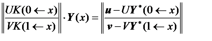
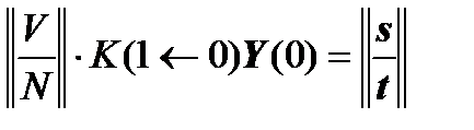
That is, we obtain two matrix equations of boundary conditions transferred to the point  under consideration:
 ,
,
 .
.
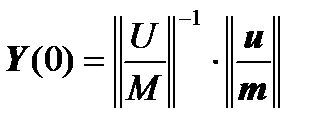
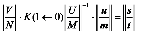
These equations are similarly combined into one system of linear algebraic equations with a square matrix of coefficients to find the solution  at any point under consideration:
 .
.
Chapter 4. The method of "additional boundary value conditions" for solving boundary value problems with non-stiff ordinary differential equations.
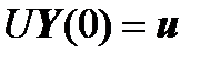
Let us write on the left edge one more equation of the boundary conditions:
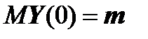 .
.
As matrix  rows, we can take those boundary conditions, that is, expressions of those physical parameters that do not enter into the parameters of the boundary conditions of the left edge
  or are linearly independent with them. This is entirely possible, since for boundary value problems there are as many independent physical parameters as the dimensionality of the problem, and only half of the physical parameters of the problem enter into the parameters of the boundary conditions.
That is, for example, if the problem of the shell of a rocket is considered, then on the left edge 4 movements can be specified. Then for the matrix  we can take the parameters of forces and moments, which are also 4, since the total dimension of such a problem is 8.
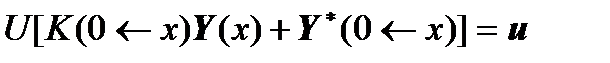
The vector  of the right side is unknown and it must be found, and then we can assume that the boundary value problem is solved, that is, reduced to Cauchy’s problem, that is, the vector
  is found from the expression:
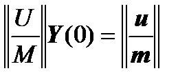 ,
,
that is, the vector is found from the solution of a system of linear algebraic equations with a square non-degenerate coefficient matrix consisting of blocks and  .
.
Similarly, we write on the right edge one more equation of the boundary conditions:
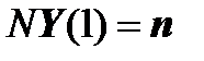 ,
,
where the matrix  is written from the same considerations for additional linearly independent parameters on the right edge, and the vector
  is unknown.
For the right edge, too, the corresponding system of equations is valid:
 .
.
We write 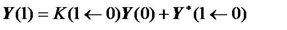 and substitute it into the last system of linear algebraic equations:
 ,
,
 ,
,
 ,
,
 .
.
We write the vector  through the inverse matrix:
and substitute it in the previous formula:
Thus, we have obtained a system of equations of the form:
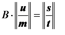 ,
,
where the matrix  is known, the vectors
  and
and  are known, and the vectors
  and
and  are unknown.
We divide the matrix into 4 natural blocks for our case and obtain:
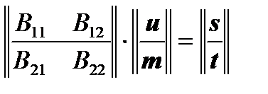 ,
,
from which we can write that
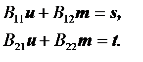
Consequently, the required vector is calculated by the formula:
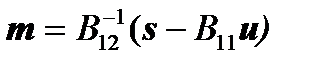
And the required vector  is calculated through the vector :
 ,
,
 .
.