
Chapter 2. Improvement of S.K.Godunov’s method of orthogonal sweep for solving boundary value problems with stiff ordinary differential equations.


2.1. The formula for the beginning of the calculation by S.K.Godunov’s sweep method.
Let us consider S.K.Godunov’s sweep method problem.
Suppose that we consider the shell of the rocket. This is a thin-walled tube. Then the system of linear ordinary differential equations will be of the 8th order, the matrix  of coefficients will have the dimension 8x8, the required vector-function
  will have the dimension 8x1, and the matrices of the boundary conditions will be rectangular horizontal dimensions 4x8.
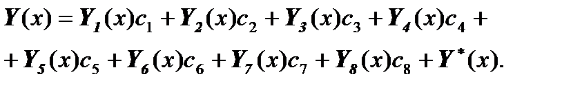
Then in S.K.Godunov’s method for such a problem the solution is sought in the following form [Godunov]:
 ,
,
or it can be written in the matrix form:
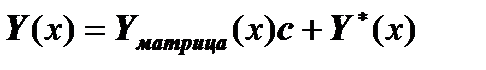 ,
,
where vectors  are linearly independent vector-solutions of the homogeneous system of differential equations, and the vector
  is a vector of a particular solution of the inhomogeneous system of differential equations.
Here 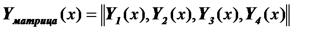 is the matrix of dimension 8x4, and
  is the corresponding vector of dimension 4x1 with the required constants
  .
.
But in general, the solution for such a boundary-value problem with dimension 8 (outside the framework of S.K.Godunov's method) can consist not of 4 linearly independent vectors , but entirely of all 8 linearly independent solution vectors of the homogeneous system of differential equations:
And just the difficulty and problem of S.K.Godunov’s method is that the solution is sought with only half the possible vectors and constants, and the problem is that such a solution with half the constants must satisfy the conditions on the left edge (the starting edge for the sweep) for all possible values of the constants, in order to find these constants from the conditions on the right edge.
That is, in S.K.Godunov’s method, there is a problem of finding such initial values  of the vectors
  , so that you can start the run from the left edge
  = 0, that is, that the conditions
  on the left edge are satisfied for any values of the constants .
Usually this difficulty is "overcome" by the fact that differential equations are written not through functionals, but through physical parameters and consider the simplest conditions on the simplest physical parameters so that the initial values can be guessed. That is, problems with complex boundary conditions can not be solved in this way: for example, problems with elastic conditions at the edges.
Below we propose a formula for the initiation of computations by S.K.Godunov’s method.
We perform the line orthonormalization of the matrix equation of the boundary conditions on the left edge:
,
where the matrix  is rectangular and horizontal dimension 4x8.
As a result, we obtain an equivalent equation of boundary conditions on the left edge, but already with a rectangular horizontal matrix  of dimension 4x8, which will have 4 orthonormal rows:
 ,
,
where, as a result of orthonormalization of the matrix , the vector  is transformed into the vector
  .
.
How to perform line orthonormation of systems of linear algebraic equations can be found in [Berezin, Zhidkov].
We complete the rectangular horizontal matrix to a square non-degenerate matrix  :
:
 ,
,
where a matrix  of dimension 4х8 must complete the matrix to a non-degenerate square matrix of dimension 8х8.
As matrix rows, we can take those boundary conditions, that is, expressions of those physical parameters that do not enter the parameters of the left edge or are linearly independent with them. This is quite possible, since for boundary value problems there are as many linearly independent physical parameters as the dimensionality of the problem, that is, in this case there are 8 of them, and if 4 are given on the left edge, then 4 can be taken from the right edge.
We complete the orthonormalization of the constructed matrix , that is, we perform the line orthonormalization and obtain a matrix  of dimension 8x8 with orthonormal rows:
 .
.
We can write down that
 .
.
Then, substituting in the formula of S.K. Godunov’s method, we get:

or
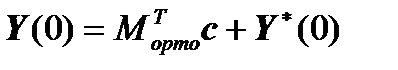 .
.
We substitute this last formula into the boundary conditions and obtain:
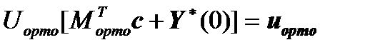 .
.
From this, we obtain that on the left-hand side the constants  no longer influence anything, since
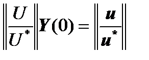
 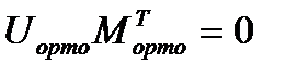 and it remains only to find the vector
  from the expression:
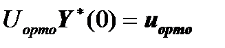 .
.
But the matrix  has a dimension of 4x8 and it must be supplemented to a square non-degenerate one in order to find the vector
  from the solution of the corresponding system of linear algebraic equations:
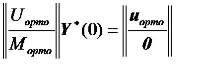 ,
,
where  is any vector, including a vector of zeros.
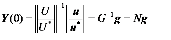
Hence we obtain by means of the inverse matrix:
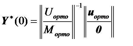 .
.
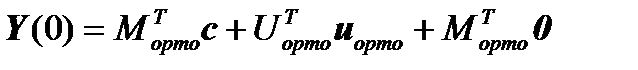
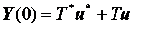
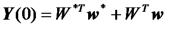
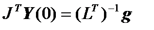
Then the formula for starting the computation by S.K. Godunov's method is as follows:
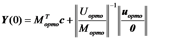 .
.
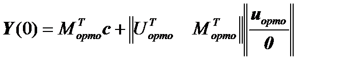
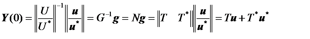
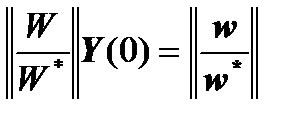
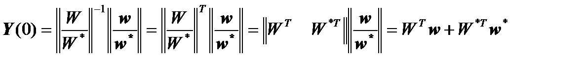
From the theory of matrices [Gantmakher] it is known that if the matrix is orthonormal, then its inverse matrix is its transposed matrix. Then the last formula takes the form:
 ,
,
 ,
,
 ,
,
 .
.
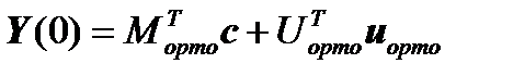
The column vectors of the matrix  and the vertical convolution vector
  are linearly independent and satisfy the boundary condition .
2.2. The second algorithm for the beginning of the calculation by S.K.Godunov’s sweep method.
This algorithm requires the addition of a matrix of boundary conditions  to a square non-degenerate one:
 .
.
The initial values are found from the solution of the following systems of linear algebraic equations:
 ,
,
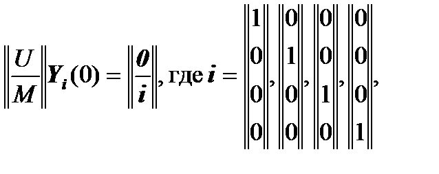
where  is a vector of zeros of dimension 4х1.
The column vectors  and the column vector
  are linearly independent and, taking part in the formation of the vector
  , satisfy the boundary condition .
2.3. The replacement of the Runge-Kutta’s numerical integration method in S.K.Godunov’s sweep method.
In S.K.Godunov's method, as shown above, the solution is sought in the form:
 .
.
At each specific section of S.K.Godunov's method of sweeping between points of orthogonalization one can use the theory of matrices instead of Runge-Kutta’s method and perform the calculation through Cauchy’s matrix:
 .
.
So perform calculations faster, especially for differential equations with constant coefficients, since in the case of constant coefficients it is sufficient to calculate once Cauchy’s matrix in a small section and then only multiply by this once computed Cauchy’s matrix.
Similarly, through the theory of matrices, we can also calculate the vector  of a particular solution of an inhomogeneous system of differential equations. Or, for this vector, Runge-Kutta’s method can be used separately, that is, one can combine the theory of matrices and Runge-Kutta’s method.
2.4 Matrix-block realizations of algorithms for starting calculation by S.K.Godunov’s sweep method.
We consider a system of linear algebraic equations expressing the boundary conditions for x=0
Suppose that there is a constructed quadratic nondegenerate matrix  .
.
Similarly, we write a vector  where the introduced vector
  is unknown.
We write the system of linear algebraic equations

or in block form
 .
.
It follows that
 .
.
Imagine 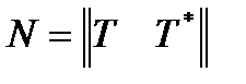 .
.
Then
 .
.
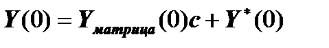
At the same time, we remember that the solution of the boundary value problem is sought in the form
 .
.
Comparing
 and
and 
given that here the vector of unknown constants is  , we obtain the initial values of the vectors for the beginning of integration in S.K.Godunov’s method.:
 и
и  .
.
Another matrix derivation can be stated in the following form.
We transform the system
by line orthonormalization to an equivalent system with orthonormal rows
 .
.
Then we can write
 .
.
Making a comparison of two expressions:
and from what  is a vector of unknown constants, we get:
 и
и  .
.
Note that another matrix-block derivation of the formulas is possible.
Transition from the system
to the system
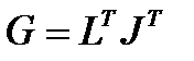
can be realized by another method, replacing the line orthonormation of by the following orthonormal decomposition of the matrix G
where the matrix J has orthonormal columns, and the matrix L is upper triangular.
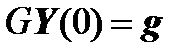
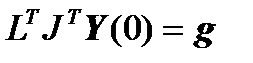
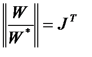
Then, taking into account the rule of transposition of matrices, we can write
 .
.
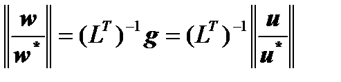
As a result, we get
 ,
,  ,
, 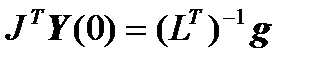 .
.
Here the rows of the matrix are orthonormal.
Comparing
and
we get
 ,
,  .
.
Thus, we again obtain the orthonormal initial values of the unknown vector-valued functions of the solution.
2.5. Conjugation of parts of the integration interval for S.K.Godunov’s sweep method.
To automate the computational process on the entire integration interval, which is composed for conjugate shells with different physical and geometric parameters, the deformation of which is described by different functions, it is necessary to have the procedures of conjugation of the corresponding functions.
In the general case, the resolving functions of various parts of the integration interval of the problem have no physical meaning, and the physical parameters of the problem are expressed in various ways through these functions and their derivatives. At the same time, conjugation of adjacent sections must satisfy kinematic and force conditions at the point of conjugation.
Solve the problem of conjugating parts of the interval of integration in the following way.
The vector P containing the physical parameters of the problem is formed using the matrix M of coefficients and the required vector-function Y(x):
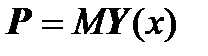
where M is a square nondegenerate matrix.
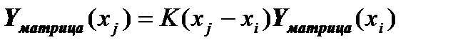
Then at the conjugation point x = x* we can write expression
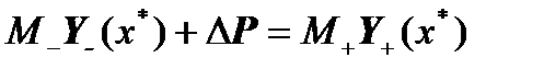 ,
,
where  is the vector corresponding to a discrete change in the physical parameters when passing through the conjugation point from the left to the right; index "-" means "to the left of the conjugation point", and the index "+" means "to the right of the conjugation point".
In S.K.Godunov’s method, the vector-function  of the problem on each section is sought in the form

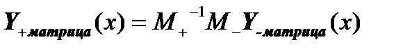
Suppose that the conjugation point does not coincide with the point of the orthogonal transformation. Then the expression for conjugation conditions of adjacent sections

will take the form
 .
.
If now demand
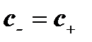
then in the direct course of the sweep method, the integration can be continued from the left to the right in the following expressions:
 ,
,
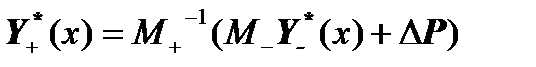 .
.
2.6. Properties of the transfer of boundary value conditions in S.K.Godunov’s sweep method.
When solving a boundary-value problem for a system of "stiff" linear ordinary differential equations by S.K.Godunov’s method says that discrete orthogonalization is carried out by Gramm-Schmidt’s method with respect to vector-functions forming the variety of solutions of the given problem in order to overcome the tendency of degeneration of these vector-functions into linearly dependent ones.
At the same time, in the implementation of S.K.Godunov’s method, the boundary conditions from the initial boundary are also transferred to the other edge. Let us show the properties of this transfer.
Previously recorded
и .
Then we can say that:
- the vector w*, which is unknown, is a vector of constants c,
- at the same time, the vector w* has the physical meaning of an external influence on the deformed system unknown at the edge x=0,
- the matrix W* is the matrix of boundary conditions unknown on the boundary x=0.
It follows from the formulated propositions that the transfer of boundary conditions in S.K.Godunov’s method has the following meaning.
The continuation of integration, beginning with the vector , means the transfer of the "convolution"  of the matrix equation of the boundary conditions at x=0 to the right edge x=1.
The continuation of the integration, beginning with the vectors in the matrix  , means that the matrix of the boundary conditions W*, which are unknown at the edge x=0, is carried to the edge x=1.
Integration of differential equations is carried out with the goal of transferring the vector c to the edge x=1, and hence the vector w*, which expresses the conditions unknown at the edge x=0.
The transfer of the matrix W* and the vector w* means that the matrix equation  of the boundary conditions, which are unknown at the edge x=0, is carried to the edge x=1.
2.7. Modification of S.K.Godunov’s sweep method.
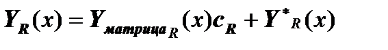
The solution in S.K.Godunov’s method is sought, as written above, in the form of the formula
.
We can write this formula in two versions - in one case the formula satisfies the boundary conditions of the left edge (index L), and in the other - the conditions on the right edge (index R):
 ,
,
 .
.
At an arbitrary point we have
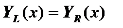 .
.
Then we obtain
 ,
,
 ,
,
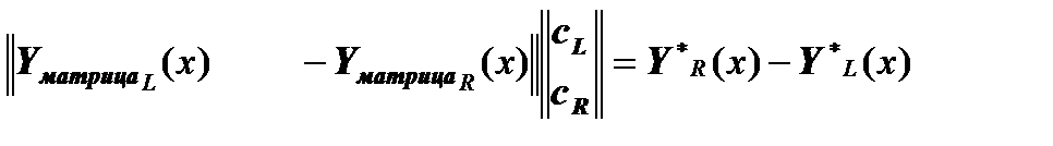 .
.
That is, a system of linear algebraic equations of the traditional kind with a square matrix of coefficients 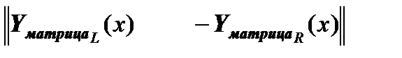 for the computation of the vectors of constants
  is obtained.